Constraint Solving with S3
Optimizing Placement of Railway Balises
As introduced in S3 Workflow, the S3 solution provides tools for a SAT-based verification of critical systems. The usual workflow for such a verification is to write an HLL model representing the critical system, and proof obligations representing the safety properties. S3 then provides the user with the appropriate tools to find counterexamples to these safety properties, if such counterexamples exist.
However, a secondary use for a SAT-based model checker such as S3 is constraint solving: given a set of constraints, S3 can provide an assignment of its variables (a.k.a. counterexample). This article describes a use case of S3 as a constraint solver in a railway signaling common problem: placing balises on a railway network, with safety constraints.
The “negative” use of S3 
How does it work?
Our approach to SAT-based constraint solving relies on one basic idea: although a SAT solver such as S3 is built to prove properties, it is equally efficient at providing counterexamples. This is simply because of how SAT solvers work: a SAT solver will either find an assignment for its variables such that the proof obligation evaluates to false, or find that the proof obligation is valid.
For now, we have only experimented with static problems (i.e.: without any temporality), hence we will only describe this range of use cases. This means that no latches are used in the HLL models in this article, and only one strategy is needed: Bounded Model Checking with depth set to 0.
In order to use S3 as a constraint solver, the basic workflow is the following.
Write an HLL model where every variable of the problem is an input, every data wished to be computed is an output, and the set of constraints is defined through an HLL definition, noted \(C\).
Set one proof obligation \(\neg{C}\).
Expand HLL to LLL using the
expand1tool, and ask S3 to analyse the one and only proof obligation.Hopefully, S3 will find a counterexample, which in this case is the result of your constraint solving.
Use
cex-simulatororwhyto make your result usable.
Here is an illustration of how we can use this to solve a famous constraint solving problem: the mighty sudoku.
The following HLL contains the variables of the problem (the numbers grid), and defines the set of constraints expressing the rules (via the definition of the boolean \(C\)), and the proof obligation \(\neg{C}\) is added:
inputs:
  int [1,9] grid_i [9,9];
declarations:
  int [1,9] grid [9,9];
definitions:
  grid[i,j] := (i+1,j+1
    | 1,1 => 1 | 1,9 => 6 | 2,3 => 6 | 2,5 => 2 | 2,7 => 7
    | 3,1 => 7 | 3,2 => 8 | 3,3 => 9 | 3,4 => 4 | 3,5 => 5
    | 3,7 => 1 | 3,9 => 3 | 4,4 => 8 | 4,6 => 7 | 4,9 => 4
    | 5,5 => 3 | 6,2 => 9 | 6,6 => 4 | 6,7 => 2 | 6,9 => 1
    | 7,1 => 3 | 7,2 => 1 | 7,3 => 2 | 7,4 => 9 | 7,5 => 7
    | 7,8 => 4 | 8,2 => 4 | 8,5 => 1 | 8,8 => 7 | 8,9 => 8
    | 9,1 => 9 | 9,3 => 8 |_,_   => grid_i[i,j]);
definitions:
  C :=
    ALL value:[1,9] (
      ALL line:[0,8] SOME col:[0,8] (grid[line, col]=value)
      & ALL col:[0,8] SOME line:[0,8] (grid[line, col]=value)
      & ALL subregion_line:[0,2], subregion_col:[0,2]
          SOME s_line:[0,2], s_col:[0,2]
            (grid[subregion_line * 3 + s_line, subregion_col * 3 + s_col]=value)
    );
proof obligations:
  ~C;
outputs:
  grid;
Here, the use of S3 (on depth 0 BMC) and one of the two counterexample analysis tool
will give the user a solution to this constraint solving problem: a valid grid.
For
instance, here is the (cut-down) output of why:
[depth 0]> grid
grid is a composite
$1: grid[0, 0] is [1]
$2*: grid[0, 1] is [2]
$3: grid[0, 2] is [3]
$4: grid[0, 3] is [7]
[...]
$78: grid[8, 5] is [5]
$79: grid[8, 6] is [3]
$80: grid[8, 7] is [1]
$81: grid[8, 8] is [2]
If, for any reasons, the constraints are too strong to be satisfied (for instance, one cell of the sudoku grid is filled with a wrong number), this will be detected: S3 will not find any counterexample and will simply return that the proof obligation is valid.
Placing Balises on a Railway
Context
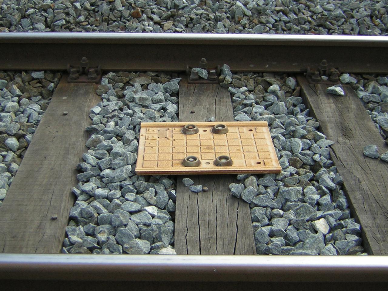
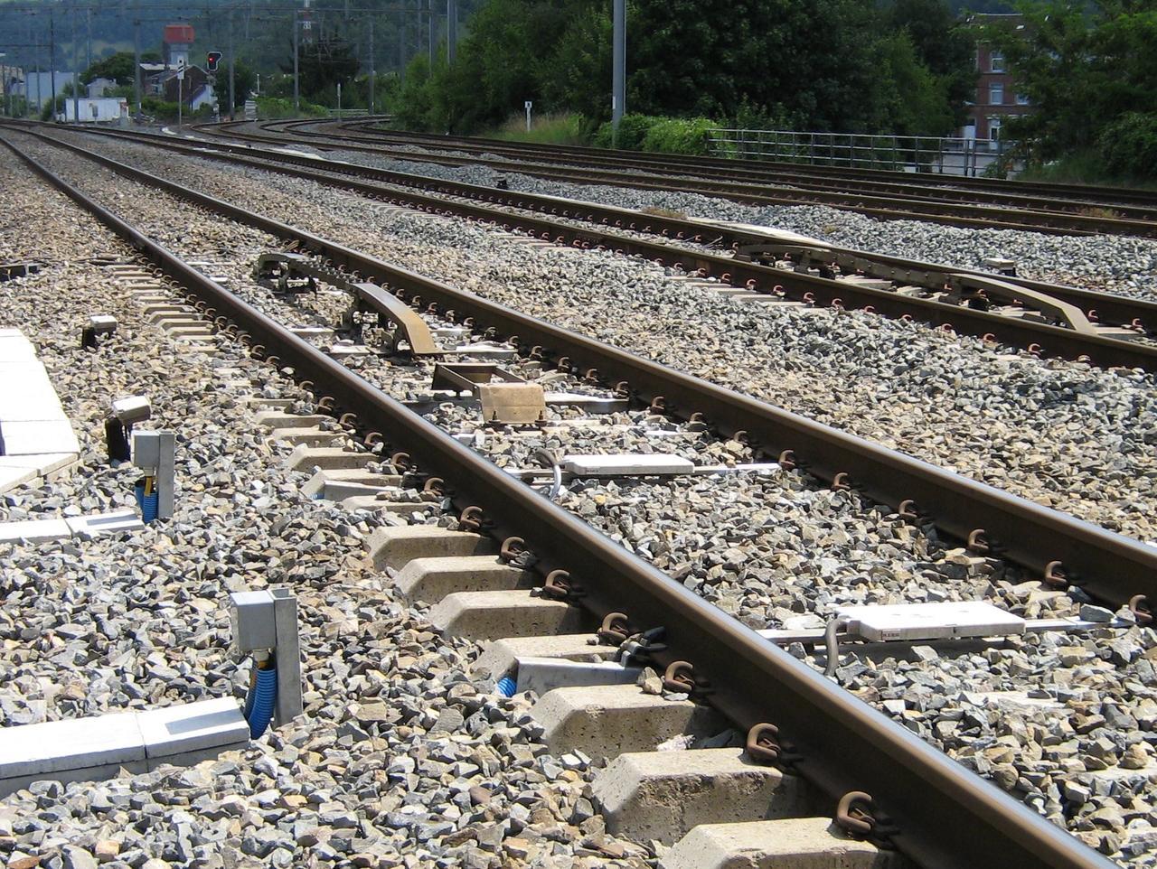
A railway balise or “balise” (CC-BY-SA Santiago Martínez Aznar)
Modern train control system like ETCS or CBTC often use balises (see Balise article on wikipedia ) placed between the rails in order to give a train its exact location, and to resynchronize its location when approaching sensitive areas.
The placement of those balises shall respect a great number of constraints such as:
at least one balise should be found inside a given range from some location (before a signal or a point),
a minimum distance should be left between two balises (or else the radio signals may interfere),
a maximum distance should be allowed between two balises (or else the train location may become too imprecise),
balises should not be placed in some exclusion zones (because of some physical impossibility),
…
Although we tackled all of these constraints kinds, this article only describes how we solved the first one.
Using S3 constraint solving capability seems a good match to solve this problem.
Proposed Solution
The balise placement problem has two input data, the first one is the description of the network:
a sort of \(N\) segments, named
t_segments, to which the itemNoneis added;a function returning the length of a given segment, noted
length;four functions
upstream1,upstream2,downstream1anddownstream2, returning upstream and downstream segments for a given segment (these functions can returnNoneif a segment has only one upstream/downstream neighbour, or no neighbour at all);
The second input is the set of constraints, meaning the safety rules that our balise placement must fulfill. The goal here is to express a boolean constraint \(C\) which negation will be added as a proof obligation in the final HLL model, much like in the sudoku solver.
In this case, constraints were basically all of the same kind: each constraint required the presence of at least one balise, upstream of a singularity of the railway network. Since these constraints were generic, we have defined a generic way to express them:
a set of \(K\) singularities
t_sing, with two functionssing_segandsing_absreturning respectively their segment and abscissa on this segment;a set of \(J\) constraints
t_cstr, and three more functions:cstr_sing,cstr_dir,cstr_dmin,cstr_dmax?.
Basically, the semantic of a constraint is: at least one balise is placed at a distance of cstr_dmin to cstr_dmax of the singularity cstr_sing, in direction
cstr_dir. Should there be a point between the singularity and the balise, then a
balise should be found on all accessible segments, always in the right distance interval.
This generic description of the constraints was done in collaboration with our client, and tailored so that every safety rule could be encoded this way. The following partial HLL summarises our actual model:
inputs:
  // how many balises are used on each segment (16 balises are allowed at most):
  [0,16] n_max_balise(t_segments);
  // abscissas of the balises on a given segment:
  int [0,MAX_SEG_LENGTH] balise_abscissa(t_segments)[16];

declarataions:
  // this function, defined in our generic part, looks for all balises
  // in the designated area, and ensures that at last one balise is
  // found on every possible path
  bool cstr_exists(T_SEGMENTS,T_SENS,T_LG_CSTR,T_LG_CSTR);

definitions:
  C :=
   ALL c:t_cstr (
     cstr_exists(
       sing_seg(cstr_sing(c)),
       cstr_sens(c),
       cstr_dmin(c) + sing_abs(cstr_sing(c)),
       cstr_dmax(c) + sing_abs(cstr_sing(c))
     )
   );

proof obligations:
  ~C;

outputs:
  n_max_balises;
  balise_abscissa;
Note that most of the HLL model is generic, and only the problem inputs described sooner (network description and constraints) need to be provided.
Once this model is assembled, with the use of the S3 solution, as described sooner, we can extract one possible assignment of our outputs: the number of balise for each segment, and the abscissa for each of those balises. This can be easily translated in our client’s desired format.
There is, however, a notable problem to this approach so far: unlike the game of sudoku, the solution to this problem is not unique, and our approach will not necessarily return the best solution. On the contrary, fulfilling every constraints seems easier if you use more balises than needed. This is were the second part our our approach kicks in.
Selecting the best solution to a constraint problem
The major flaw to our constraint solving approach so far, is that we cannot select which solution will be returned out of the many possible solutions. A SAT-solver based model checker such as S3 will look at any solution, and stop at the first one.
This is why we needed to provide a way to select the best solution. We did so by using
another tool from the S3 toolbox: cex-selector. This tool can be used to select
a counterexample found by S3, out of the many possible counterexamples. The selection can
be done thanks to the use of custom metrics (given in HLL): basically, this tool uses S3
iteratively, in order to minimize those metrics.
In that case, the total amount of balises used seems like a good metric, for obvious economical reasons.
The tool cex-selector takes as input a metrics file. The following is the metric used
for the balise placement problem:
nof_balise:
- minimum
- int : SUM s:t_segments (n_max_balise(s));
- range : 500..1500
Here, we use only one metric (nof_balise). The user can give a hint of what he believes
the optimal is in order to make the search faster: here between 500 and 1500 balises
(that hint can be checked by cex-selector, or left empty if unsure). If needed,
it is possible to add subsequent metrics, in which case each metric will be
minimised while keeping every previous metric at their optimal (lexicographic ordering).
Finally, using an iterative approach, with S3 used over multiple threads,
cex-selector will look for the best solution. Since S3 is a certified tool,
we can tell with certainty that there is no better solution: any other solution will use
at least as many balises.
This has been completed on two different subway lines, requiring little to no work to adapt to the second one. Each “balise problem” was successfully solved in under 15 minutes.
What more can it do?
This first result seems satisfying, but some other needs have to been fulfilled. Here is a quick list of improvements that have been done since this first step, or could be.
Successive iterations
Although the use of constraint solving to compute balise locations is a time saver in itself, it is at least as important to ensure that maintenance can be done just as efficiently. If for any reason, the balise placement needs to be reevaluated (mostly updated safety rules), we will need to find another solution, but possibly while keeping the balises already installed. This kind of flexibility is possible thanks to the descriptive nature of HLL: it is always possible, and relatively simple, to add these new constraints to the HLL model. It is also possible to fix a part of the variables, for instance to ensure that the installed balises will not need moving.
This possibility for successive iterations solves an other of our client risk: if for some reason, the installation of a balise was physically impossible at the chosen location, it is always possible to make another iteration with a “forbidden” area.
These iterations take a similar time as the initial run, and this is where we believe most of the time and money can be saved: the old fashion way was to manually update the balise placement, which becomes increasingly complicated.
Traceability
One of the biggest inconvenient was initially traceability, since our approach does not naturally provide an explanation for each balise location: it is only here because the whole solution is valid according to the entire model.
It was however easy by enriching the HLL model to compute a traceability matrix, linking every balise to the constraints that have an influence on its location. This matrix is not a one to one relation between constraints and balises, and that’s for the best: it allows to find solution with way less balises than constraints, by regrouping many overlapping constraints.

Diagrams of balises (purples) with all their constraints (click to zoom).
Commentaires